Throughout a startup’s lifecycle, its business model, cash flows, and nature of operations keep evolving. Initially, many startups focus primarily on research and development. As they grow and reach key milestones, they begin generating regular revenue, attracting investor interest, and expanding operations to include product development, customer acquisition, and marketing.
By the latter stage of a startup’s lifecycle, it will have turned into a completely different organization from how it began. It would serve a broader customer base across diverse geographies and product lines, with technologies attractive to a wider range of large corporations. Thus, as its scale increases, so will its relevance in the mergers and acquisitions (M&A) market. Hence, throughout your startup’s lifecycle, you must continually update your fair value measurement techniques.
This article will discuss startups’ lifecycle stages, how they should choose valuation approaches and techniques in each stage, and explain all valuation techniques recommended under ASC 820.

When do startups need to comply with ASC 820?
The documentation for ASC 820 does not specify when it needs to be followed. Instead, when other accounting standards require fair value measurement, you must follow the guidelines of ASC 820. The most relevant scenarios that follow ASC 820 guidelines are acquisitions and startup valuations for stock-based compensation.
Under ASC 805, the acquired business’s assets, liabilities, goodwill, and noncontrolling interests, as well as bargain purchase gains, must be recognized at fair value. Furthermore, under ASC 718, stock-based compensation expenses must be recognized at fair value.
Additionally, you may need to be mindful of ASC 820 when you report values of derivatives, financial instruments, long-lived assets, and indefinite-lived assets.
Which valuation approaches are applicable at different stages of a startup’s lifecycle?
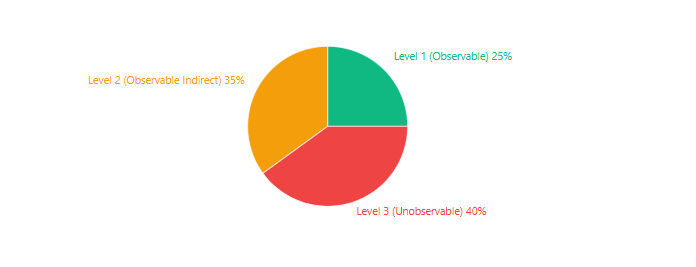
At any stage in a startup’s lifecycle, when it comes to asset valuation, you must choose an approach that is most suitable for that asset. The Fair Value Measurement standard recommends choosing approaches that minimize dependence on unobservable inputs and focus on observable inputs. Let’s explore which approach and technique are most suitable for each startup lifecycle stage.
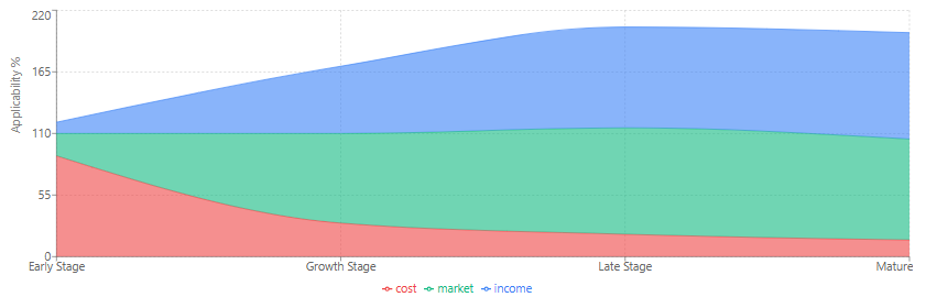
Early stage
In the early stages of a startup’s lifecycle, it is unlikely to have stable revenue, so the income approach is unusable at this stage. Many startups also operate in stealth mode to maintain secrecy regarding their business ideas and technologies. In this startup lifecycle, a startup rarely becomes an acquisition target. Hence, the market approach cannot be applied due to the lack of data.
As a result, an early-stage startup may have to rely on the cost approach for ASC 820 reporting.
Growth stage
When a company reaches the growth stage of the startup lifecycle, it may fetch a much higher valuation in funding rounds and have overcome significant challenges and achieved key milestones. Hence, instead of using the cost approach, you may get better results through the market approach.
If abundant data regarding comparable transactions exists, you could use the market valuation multiple techniques. You could also use the comparable company technique if companies with similar business models and geographical diversification exist.
You must exercise extreme care when valuing growth-stage startups through the income approach during this phase of the startup lifecycle. A startup may correctly assume high growth rates but overlook the need to make reasonable discount rate assumptions that incorporate the inherent risks associated with such growth.
Option pricing models may prove to be a more appropriate income approach technique because of their ability to capture the uncertainty of future outcomes.
Late stage
By the time a company reaches the late stage of the startup lifecycle, it is likely to have a broad range of competitors. Thus, there would be ample data on how venture capitalists value similar companies. This makes it easier to build reliable market valuation multiples.
For the same reason, the comparable company method also delivers accurate results.
Since companies tend to have a fairly long financial history and stable revenue at this startup lifecycle stage, the income approach, too, has high applicability. The abundance of data makes it easier to build reliable financial forecasts without incorporating too many unobservable inputs.
The cost approach is not appropriate for late-stage startups for the same reason it is not appropriate for growth-stage startups.
Valuation approaches and techniques recommended under ASC 820?
Under ASC 820, you must follow the income, cost, and market approaches to valuation depending on the startup lifecycle stage. In this section, we will discuss the recommended valuation techniques coming under these approaches and when to use them.
Income approach
Under the income approach, an asset or a company’s value is determined based on the cash flows it is expected to generate. To account for risk and inflation, we often apply a discount rate in this approach.
The most well-known technique is the discounted cash flow (DCF) method which is commonly used for company valuations in the later stages of startup lifecycle. This is useful especially when financial data is abundant, involves preparing cash flow projections, discounting them, and summing them up to find the asset’s valuation.
Suppose an asset is expected to generate a net income of $800,000 every year for 10 years, after which its resale value would be $1.6 million. Assuming a discount rate of 15%, we can calculate the value of this asset as:
| Year | Income (A) | Discounting factor (B) | Present value (C = A÷B) |
|---|---|---|---|
| 2025 | $800,000 | 1.15 | $695,652 |
| 2026 | $800,000 | 1.3225 | $604,915 |
| 2027 | $800,000 | 1.520875 | $526,013 |
| 2028 | $800,000 | 1.74900625 | $457,403 |
| 2029 | $800,000 | 2.011357188 | $397,741 |
| 2030 | $800,000 | 2.313060766 | $345,862 |
| 2031 | $800,000 | 2.66001988 | $300,750 |
| 2032 | $800,000 | 3.059022863 | $261,521 |
| 2033 | $800,000 | 3.517876292 | $227,410 |
| 2034 | $800,000 | 4.045557736 | $197,748 |
| 2034 (Resale value) | $1,600,000 | 4.045557736 | $395,496 |
| Asset value (Total) | $4,410,510 |

Option pricing models are also well-known income approach valuation techniques. They treat an asset or company as a financial option to capture the present value of future economic benefits by adjusting for risk in uncertain environments. The Black-Scholes model is often used to determine the value of complex securities, patents, research and development projects, as well as equity.
Suppose you own a pharma startup, and you have an opportunity to develop a patent for a medicine. The present value of the income expected to be generated by this patent is $20 million. The cost of developing this patent is $8 million, and you have 2 years to decide whether to develop such a patent. Based on market research, you can expect a volatility of 30%. At present, the US Fed is maintaining an interest rate of 4.5%.
In this scenario, you can calculate the value of this patent by assigning the following values to the key variables in the Black-Scholes call option pricing formula.
- Exercise price = Required investment = $8 million
- Current price = Present value of expected future cash flows = $20 million
- Risk-free interest rate = US Federal Funds Rate = 4.5%
- Time to maturity = Time available to make the decision = 2 years
- Volatility = 30%
When you input these values in the Black-Scholes call option pricing model, you will arrive at $12.7 million as the patent valuation.
To calculate the intangible assets using the income approach, you can use the valuation technique called the multiperiod excess earnings method (MEEM). In this technique, we separate cash flows attributable to the asset being valued by subtracting contributory charges for other assets. Let us understand this technique through an example.
Suppose you must value your brand. The brand power that you have accumulated thus far is expected to last 5 years. In this period, your company is expected to generate an annual operating income of $400,000 every year. The expected tax rate is 25%. Your internal research tells you that your fixed assets and workforce contribute 20% and 40% of your operating income, respectively. Assuming a discount rate of 15%, you can calculate the value of your brand as follows:
Step 1: Calculating the excess income after tax
| Particulars | Amount |
|---|---|
| Annual operating income | $400,000 |
| Income attributable to fixed assets (20% of A) | $80,000 |
| Income attributable to the workforce (40% of A) | $160,000 |
| Excess income (A-B-C) | $160,000 |
| Tax on excess income (25% of D) | $40,000 |
| Excess income after tax (D-E) | $120,000 |
Step 2: Discounting the excess income after tax
| Year | Excess income after tax (A) | Discounting factor (B) | Present value (C=A÷B) |
|---|---|---|---|
| 2025 | $120,000 | 1.15 | $104,348 |
| 2026 | $120,000 | 1.3225 | $90,737 |
| 2027 | $120,000 | 1.520875 | $78,902 |
| 2028 | $120,000 | 1.74900625 | $68,610 |
| 2029 | $120,000 | 2.011357188 | $59,661 |
| Asset value (Total) | $402,259 |
Cost approach
The cost approach, generally reserved for early stages of startups’ lifecycle, simply assigns the cost of replacing or rebuilding an asset as its valuation. This approach is typically used for replaceable assets such as vehicles, plant, and machinery.
Suppose you need to report the fair value of a fleet of 20 identical commercial vehicles. In the used vehicles market, one such unit sells for $50,000. Then, the valuation of this fleet of commercial vehicles would be $1,000,000 (20 × $50,000).
Market approach
In the market approach, we estimate an asset’s value based on the market value of comparable assets. In company valuation, a commonly used market approach valuation technique is the comparable company method.
Here, you must apply a comparable company’s valuation multiple to the financial performance of your company and make adjustments for differences in scale, growth prospects, and risk profile.
Suppose your startup has an EBITDA of $30 million. A company with a similar business model has an EV/EBITDA ratio of 16. Assume that you need to apply a discount of 20% to account for the difference in scale, growth prospects, and risk profile.
Then, as per the comparable company method, your company’s valuation can be calculated as:
| Particulars | Amount |
|---|---|
| EBITDA | $30,000,000 |
| EV/EBITDA ratio | 16 |
| Pre-adjustment valuation (A×B) | $480,000,000 |
| Discount rate | 20% |
| Valuation (C×(1-D)) | $384,000,000 |
Another company valuation technique under this approach is the market valuation multiple method. Here, you must apply a market’s valuation multiple to your company’s financial performance to find its valuation.
Suppose your company has an annualized revenue of $50 million. Market research suggests that your peers have a combined annualized revenue of $500 million and a combined valuation of $13 billion.
Then, the market valuation multiple would be = $13 billion ÷ $500 million
= 26
Then, your company’s valuation would be = $50 million × 26
= $1,300,000,000
You can use the matrix pricing technique to value securities that are not actively traded. Let us see how this technique is used to value bonds.
Suppose you own a bond whose rating is AAA, face value is $1,000, maturity is 4 years, and interest rate is 5%. Market research reveals the following details about similar bonds.
| Bond | Rating | Maturity | Interest rate | Price | Yield |
|---|---|---|---|---|---|
| AAA | 3 years | 4.50% | $990 | 4.87% | |
| AAA | 5 years | 5.50% | $1,010 | 5.27% |
Now, you can use this data to estimate the yield investors would demand for the bond you hold. You can calculate this as the interpolated yield, which would form the discount rate for your bond.
Interpolatedyield
=Bond B’s yield- (Bond B’s yield-Bond A’s yield / Bond B’s maturity – Bond A’s maturity) × (Your bond’s maturity – Bond A’s maturity)
= 5.267% – (5.267% – 4.866% / 5-3) × (4-3)
≈ 5.067%
Now, let us calculate the value of all cash flows expected from the bond.
| Year | Cash flow | Discounting factor | Present value |
|---|---|---|---|
| 2025 | $50 | 1.050665 | $48 |
| 2026 | $50 | 1.103896942 | $45 |
| 2027 | $50 | 1.159825881 | $43 |
| 2028 | $50 | 1.218588459 | $41 |
| 2028 (Redemption) | $1,000 | 1.218588459 | $821 |
| Asset value (Total) | $998 |

Eqvista – Compliance with accuracy!
Compliance with ASC 820 is a key part of accurate financial reporting, which helps build positive investor relations and ensure tax compliance. However, due to the complexity and variety of techniques, you may need the assistance of experts.
Eqvista’s valuation team can provide accurate, swift, and defensible asset and company valuation reports to ease this burden. Contact us to learn more about our services!


